Introduction
Overview
Teaching: 0 min
Exercises: 0 minQuestions
What is the purpose of this course?
Objectives
We are here to learn how to implement machine learning models with
tidymodels.
What is Machine Learning?
Machine learning has received a lot of attention in recent years. It is a field of study that gives computers the ability to learn without being explicitly programmed. It is a subset of artificial intelligence (AI) and is often used to make predictions or classifications. Machine learning is used in many fields, including medicine, finance, and marketing.
Under the hood, machine learning algorithms are just a series of mathematical equations trying to find patterns in data. Once these patterns are represented in the form of a model, they can be used to make predictions or classifications on new data.
What is a Model?
A model is some sort of mathematical or logical system used to represent a real-world phenomenon. For example, a linear regression model is a mathematical equation that represents the relationship between two variables. The model can then be used to make predictions about what will happen in the future.
Models generally have some assumptions or rules that they assume are true. For example, a linear regression model assumes that the relationship between two variables is linear. If this assumption is not true, then the model will not be accurate.
When trying to model a phenomenon, it is assumed that there is some underlying process that generates the data. The model is then used to represent this process. This process or relationship is often referred to as the “structure” of the problem. As well as structure, there is also “noise” in the data. This is the random variation that is not explained by the model. Teh aim of a model is to capture the structure of the data and ignore the noise.
Parameters and Hyperparameters
A model has two types of parameters: parameters and hyperparameters. Parameters are the values that are estimated from the data. For example, in a linear regression model, the parameters are the intercept and slope. Hyperparameters are the values that are set by the user. For example, in a linear regression model, the hyperparameters are the number of variables to include in the model and the type of regression to use.
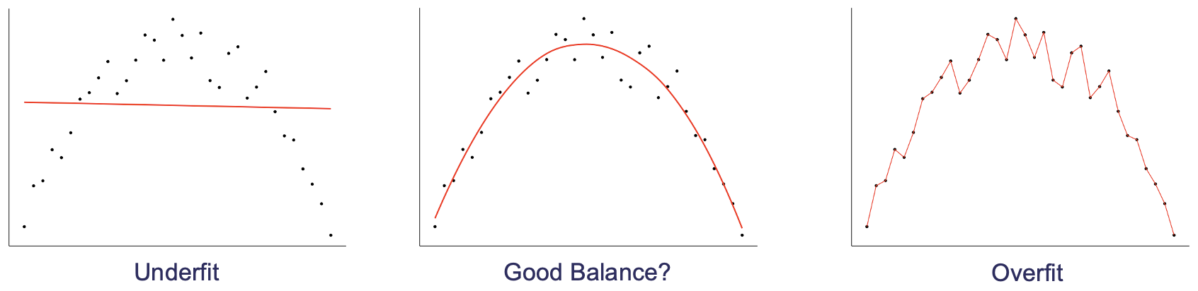
We have to be careful when choosing hyperparameters because they can have a big impact on the performance of the model. For example, if we choose too many variables to include in the model, then it will be overfit to the data and will not generalize well to new data. If we choose too few variables, then it will be underfit to the data and will not capture the structure of the data. The choice of model itself can also be considered to be a hyperparameter, so we have to be careful when choosing the model as well and make sure that it is appropriate for the problem at hand.
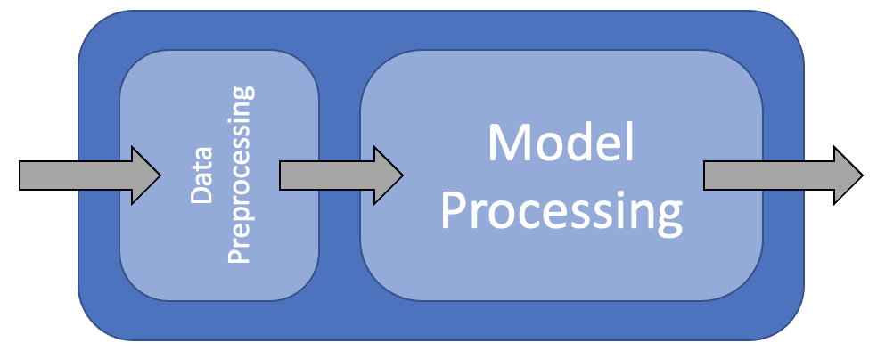
What is a Workflow?
A workflow is a series of steps that are performed in order to achieve a goal. In machine learning, a workflow is a series of steps that are performed in order to build a model. The steps in a workflow can be broken down into three categories: data preparation, model building, and model evaluation.
In this course we are going to use the tidymodels framework to build our models. The tidymodels framework is a collection of packages that are designed to work together to make it easier to build models. The packages in the tidymodels framework are:
- recipes: A package for data preparation
- parsnip: A package for specifying models
- dials: A package for tuning hyperparameters
- workflows: A package for building workflows
- yardstick: A package for model evaluation
As well as these packages, we will also be using the tidyverse packages for data manipulation and visualization.
Why use Tidymodels?
The tidymodels framework is designed to make it easier to build models. It does this by providing a consistent interface for all of the packages in the framework. This means that you can use the same code to build different types of models. For example, you can use the same code to build a linear regression model and a random forest model. This makes it easier to compare different types of models and choose the best one for your problem.
Loading Data
library(tidyverse)
library(tidymodels)
library(mlbench)
library(caret)

data(BostonHousing)
housing <- BostonHousing |>
    as_tibble()

housing |>
    glimpse()
Rows: 506
Columns: 14
$ crim    <dbl> 0.00632, 0.02731, 0.02729, 0.03237, 0.06905, 0.02985, 0.08829, 0.14455, 0.21124, 0.17004, 0.2248…
$ zn      <dbl> 18.0, 0.0, 0.0, 0.0, 0.0, 0.0, 12.5, 12.5, 12.5, 12.5, 12.5, 12.5, 12.5, 0.0, 0.0, 0.0, 0.0, 0.0…
$ indus   <dbl> 2.31, 7.07, 7.07, 2.18, 2.18, 2.18, 7.87, 7.87, 7.87, 7.87, 7.87, 7.87, 7.87, 8.14, 8.14, 8.14, …
$ chas    <fct> 0, 0, 0, 0, 0, 0, 0, 0, 0, 0, 0, 0, 0, 0, 0, 0, 0, 0, 0, 0, 0, 0, 0, 0, 0, 0, 0, 0, 0, 0, 0, 0, …
$ nox     <dbl> 0.538, 0.469, 0.469, 0.458, 0.458, 0.458, 0.524, 0.524, 0.524, 0.524, 0.524, 0.524, 0.524, 0.538…
$ rm      <dbl> 6.575, 6.421, 7.185, 6.998, 7.147, 6.430, 6.012, 6.172, 5.631, 6.004, 6.377, 6.009, 5.889, 5.949…
$ age     <dbl> 65.2, 78.9, 61.1, 45.8, 54.2, 58.7, 66.6, 96.1, 100.0, 85.9, 94.3, 82.9, 39.0, 61.8, 84.5, 56.5,…
$ dis     <dbl> 4.0900, 4.9671, 4.9671, 6.0622, 6.0622, 6.0622, 5.5605, 5.9505, 6.0821, 6.5921, 6.3467, 6.2267, …
$ rad     <dbl> 1, 2, 2, 3, 3, 3, 5, 5, 5, 5, 5, 5, 5, 4, 4, 4, 4, 4, 4, 4, 4, 4, 4, 4, 4, 4, 4, 4, 4, 4, 4, 4, …
$ tax     <dbl> 296, 242, 242, 222, 222, 222, 311, 311, 311, 311, 311, 311, 311, 307, 307, 307, 307, 307, 307, 3…
$ ptratio <dbl> 15.3, 17.8, 17.8, 18.7, 18.7, 18.7, 15.2, 15.2, 15.2, 15.2, 15.2, 15.2, 15.2, 21.0, 21.0, 21.0, …
$ b       <dbl> 396.90, 396.90, 392.83, 394.63, 396.90, 394.12, 395.60, 396.90, 386.63, 386.71, 392.52, 396.90, …
$ lstat   <dbl> 4.98, 9.14, 4.03, 2.94, 5.33, 5.21, 12.43, 19.15, 29.93, 17.10, 20.45, 13.27, 15.71, 8.26, 10.26…
$ medv    <dbl> 24.0, 21.6, 34.7, 33.4, 36.2, 28.7, 22.9, 27.1, 16.5, 18.9, 15.0, 18.9, 21.7, 20.4, 18.2, 19.9, …
Key Points
tidymodelsis a collection of packages that are designed to work together to make it easier to build models.
Machine Learning Basics
Overview
Teaching: 0 min
Exercises: 0 minQuestions
Why do we split data into training and testing sets?
When do we use validation sets?
What is cross validation?
How do we evaluate a model?
What is bias and variance?
Objectives
Revise basic concepts in machine learning
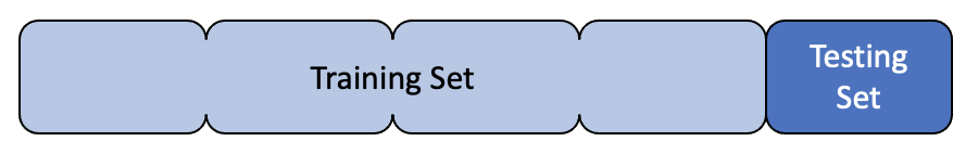
Test/Train Split
Creating a model is all well and good, but how do we know that it is actually going to be useful in the real world? Essentially, we are asking how well does our model generalise to new data? To get an estimate of this, we can split our data into two sets: a training set and a test set. We can then train our model on the training set and evaluate it on the test set. This is known as the test/train split.
What proportion of the data should be used for training?
Discuss in small groups what proportion of data should be used for training. What are the advantages and disadvantages of using more or less data for training? If you have a lot of data, is it better to use more or less for training?
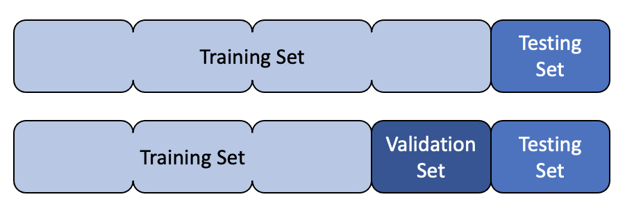
Validation Set
Let’s say we have two different models and we want to know which one to choose from, or maybe even two versions of the same type of model but with different hyperparameters, how do we know which one is best? At first this seems like a simple question, we just evaluate them on the test set and choose the one with the best performance. However, this is not a good idea. The test set is used to evaluate the final model, and so we should not use it to choose the model. If we do, we are likely to overfit to the test set and our model will not generalise well to new data.
Instead, we can split our data into three sets: a training set, a validation set and a test set. We can then train our models on the training set, evaluate them on the validation set and choose the best one. We can then evaluate the final model on the test set.
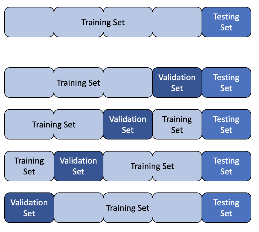
Cross Validation
Cross validation is a more advanced method for estimating the performance of a model. It is useful when we have a small dataset and we want to get a more accurate estimate of the performance of our model. It is also useful when we want to tune the hyperparameters of our model.
The basic idea is to split the data into k folds. We then train our model on k-1 folds and evaluate it on the remaining fold. We repeat this process k times, each time using a different fold for evaluation. We can then average the results to get an estimate of the performance of our model.
Model Evaluation
There are many different ways to evaluate a model. The most common are error, accuracy, confusion matrix, sensitivity and specificity. Which one you use depends on the type of problem you are trying to solve.
Error
For regression tasks, the performance of a model is usually determined by the error. There are many different types of error, but the most common is the mean squared error (MSE). This is simply the mean of the squared differences between the true values and the predicted values. The reason for squaring the differences is that it penalises large errors more than small errors.
Accuracy
Accuracy is the simplest metric for evaluating a model. For classification tasks, it is simply the proportion of predictions that are correct. For regression tasks, it is the proportion of predictions that are within a certain threshold of the true value. For example, if we are trying to predict the price of a house, we might say that the prediction is correct if it is within £10,000 of the true value.
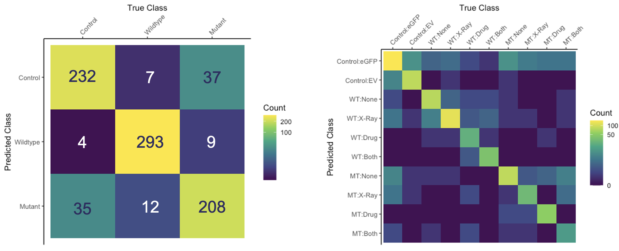
Confusion Matrix
A confusion matrix is used to visualise the performance of a classification model. It shows the number of true positives, true negatives, false positives and false negatives. It is useful for understanding where a model is going wrong. For example, if a model is predicting a lot of false positives, it might be useful to look at the false positives and see if there is a pattern. Perhaps the model is predicting a lot of false positives for a particular class, in which case it might be useful to look at the data for that class and see if there is a problem with the data.
Confusion matrices can be extended for multiclass problems. For example, if we have three classes, we can create a 3x3 matrix where the rows represent the true classes and the columns represent the predicted classes.
Sensitivity and Specificity
Sensitivity and specificity are useful metrics for evaluating models when the classes are imbalanced. For example, if we are trying to predict whether a patient has a disease or not, we might have a dataset where 99% of the patients do not have the disease and only 1% do. If we were to create a model that always predicted that the patient did not have the disease, it would be 99% accurate, but it would not be very useful. Sensitivity and specificity are useful metrics for evaluating models in these situations.
Both of these can be considered as conditional probabilities. Sensitivity is the probability that the model predicts a positive result given that the true result is positive. Specificity is the probability that the model predicts a negative result given that the true result is negative. That is to say, sensitivity is the probability of a true positive and specificity is the probability of a true negative.
Plotting sensitivity and specificity against one another is often used to produce a receiver operating characteristic (ROC) curve. The area under the ROC curve (AUC) is a useful metric for evaluating models, but is not covered in this short course.
Bias and Variance
Bias and variance are useful concepts for understanding how a model will perform on new data. Bias is the difference between the expected value of the predictions and the true value. Variance is the variability of the predictions. A model with high bias will tend to underfit the data, whereas a model with high variance will tend to overfit the data.
Thinking back to the ideas of structure and noise, we can see that bias is related to structure and variance is related to noise. A model with high bias will tend to not capture all of the structure and a model with high variance will tend to have a lot of noise.
Key Points
Testing sets are used to estimate a models performance on new data
Validation sets are used to choose between different models or hyperparameters
Cross validation is a more advanced method for estimating the performance of a model
Accuracy is a simple metric for evaluating a model
Confusion matrices are a more detailed way of evaluating a model
Precision and recall are useful metrics for evaluating models when the classes are imbalanced
Bias and variance are useful concepts for understanding how a model will perform on new data
Data Preparation
Overview
Teaching: 0 min
Exercises: 0 minQuestions
How do you split your data?
What is a recipe?
Objectives
Learn how to split your data.
Learn how to create a recipe.
Splitting Your Data
Test/Train Split
The first thing that you need to do when you have your data is to split it into a training and testing set. This is so that you can train your model on one set of data and then test it on another set of data. This is important because if you train your model on all of your data then you won’t have any data left to test it on. This means that you won’t be able to tell if your model is overfitting to your data.
housing_split <- housing |>
  initial_split(prop = 0.8)

housing_train <- training(housing_split)

housing_test <- testing(housing_split)

housing_train
# A tibble: 404 × 14
      crim    zn indus chas    nox    rm   age   dis   rad   tax ptratio     b lstat  medv
     <dbl> <dbl> <dbl> <fct> <dbl> <dbl> <dbl> <dbl> <dbl> <dbl>   <dbl> <dbl> <dbl> <dbl>
 1  0.207      0 27.7  0     0.609  5.09  98    1.82     4   711    20.1 318.  29.7    8.1
 2 11.8        0 18.1  0     0.718  6.82  76.5  1.79    24   666    20.2  48.4 22.7    8.4
 3  0.142      0  6.91 0     0.448  6.17   6.6  5.72     3   233    17.9 383.   5.81  25.3
 4  0.0883     0 10.8  0     0.413  6.42   6.6  5.29     4   305    19.2 384.   6.72  24.2
 5  0.127      0  6.91 0     0.448  6.77   2.9  5.72     3   233    17.9 385.   4.84  26.6
 6  0.0918     0  4.05 0     0.51   6.42  84.1  2.65     5   296    16.6 396.   9.04  23.6
 7  0.0178    95  1.47 0     0.403  7.14  13.9  7.65     3   402    17   384.   4.45  32.9
 8  4.67       0 18.1  0     0.713  5.98  87.9  2.58    24   666    20.2  10.5 19.0   12.7
 9  0.141      0 13.9  0     0.437  5.79  58    6.32     4   289    16   397.  15.8   20.3
10  0.0689     0  2.46 0     0.488  6.14  62.2  2.60     3   193    17.8 397.   9.45  36.2
# ℹ 394 more rows
# ℹ Use `print(n = ...)` to see more rows
Validation Splits
You can also use rsample to create validation splits. These are useful if you want to tune your model hyperparameters. You can use vfold_cv to create a validation split. This will create a number of folds (5 by default) and then repeat this a number of times (3 by default). You can then use these folds to tune your model (as wel will see in a later episode).
housing_folds <- vfold_cv(housing_train, v = 5, repeats = 3)

housing_folds
#  5-fold cross-validation repeated 3 times
# A tibble: 15 × 3
   splits           id      id2
   <list>           <chr>   <chr>
 1 <split [323/81]> Repeat1 Fold1
 2 <split [323/81]> Repeat1 Fold2
 3 <split [323/81]> Repeat1 Fold3
 4 <split [323/81]> Repeat1 Fold4
 5 <split [324/80]> Repeat1 Fold5
 6 <split [323/81]> Repeat2 Fold1
 7 <split [323/81]> Repeat2 Fold2
 8 <split [323/81]> Repeat2 Fold3
 9 <split [323/81]> Repeat2 Fold4
10 <split [324/80]> Repeat2 Fold5
11 <split [323/81]> Repeat3 Fold1
12 <split [323/81]> Repeat3 Fold2
13 <split [323/81]> Repeat3 Fold3
14 <split [323/81]> Repeat3 Fold4
15 <split [324/80]> Repeat3 Fold5
Preprocessing Your Data
Preprocessing your data should take you a really really really long time. Machine learning has a ‘garbage in = garbage out’ philosophy, which is to say that if you don’t put useful information into your model then you won’t get useful insights from your model.
Data preprocessing starts before you collect your data. When planning experiments or surveys it is important to have a clear question in mind and ensure that you collect all of the data that you need. Machine learning is often synonimised with ‘Big Data’ and therefore comes with the misconception that giving your model more data will always help it improve. Giving your model more data points (more observations) is beneficial to model performance, but there is an effect called the ‘Hughes Phenomynon” that says giving your model more variables will help to a point, but then having to deal with all of these variables will decrease the power of your model and will have a negative effect on performance.
Once you have collected your data, you might find that some (or all of) it needs transforming before it can be fed into a model. This can be done by hand, or there are ways to automate the process. To start investigating our data we can use the skimr package to create a short summary of each variable.
What Sort of Processing Might This (or a Similar) Dataset Need?
In small groups or on your own, look at the summary informations and discuss what sort of processing this data, or a similar data set might need. Remember that we will be applying our model to unseen data and this may have different properties to the data before you.
# library(skimr)

skim(housing_train)
── Data Summary ────────────────────────
                           Values
Name                       housing_train
Number of rows             404
Number of columns          14
_______________________
Column type frequency:
  factor                   1
  numeric                  13
________________________
Group variables            None

── Variable type: factor ─────────────────────────────────────────────────────────────────────────────────
  skim_variable n_missing complete_rate ordered n_unique top_counts
1 chas                  0             1 FALSE          2 0: 375, 1: 29

── Variable type: numeric ────────────────────────────────────────────────────────────────────────────────
   skim_variable n_missing complete_rate    mean      sd        p0      p25     p50     p75    p100 hist
 1 crim                  0             1   3.42    7.55    0.00632   0.0861   0.263   3.69   73.5   ▇▁▁▁▁
 2 zn                    0             1  10.4    22.5     0         0        0       3.12  100     ▇▁▁▁▁
 3 indus                 0             1  11.4     6.95    0.74      5.19     9.69   18.1    27.7   ▇▆▁▇▁
 4 nox                   0             1   0.556   0.117   0.389     0.453    0.538   0.624   0.871 ▇▇▅▃▁
 5 rm                    0             1   6.28    0.717   3.56      5.88     6.19    6.62    8.78  ▁▂▇▂▁
 6 age                   0             1  69.0    28.3     2.9      45.8     79.1    94.1   100     ▂▂▂▂▇
 7 dis                   0             1   3.78    2.11    1.13      2.10     3.17    5.14   12.1   ▇▅▂▁▁
 8 rad                   0             1   9.56    8.74    1         4        5      24      24     ▇▂▁▁▃
 9 tax                   0             1 409.    170.    187       280.     330     666     711     ▇▇▃▁▇
10 ptratio               0             1  18.5     2.20   12.6      17       19.1    20.2    22     ▁▃▃▅▇
11 b                     0             1 357.     90.4     0.32    375.     391.    396.    397.    ▁▁▁▁▇
12 lstat                 0             1  12.7     7.22    1.73      7.09    11.2    16.9    38.0   ▇▇▃▂▁
13 medv                  0             1  22.7     9.35    5        17.0     21.2    25      50     ▂▇▃▁▁
In ‘tidymodels’, we can use the ‘recipes’ package to create data preprocessing steps that can be pre-appended to the model. This means that when we give data to the model, the model will first use this recipe to transform the new observations and will then feed this tranformed data into the model and use that to make predictions.
What are the Advantages/Disadvantages of Using Data Preprocessors Over Manually Processing Data?
What are the advantages and disadvantages of using data preprocessing as part of a workflow are compared to processing new data by hand.
In this section we are going to build an extremely basic recipe to preprocess our data. You can create a recipe using the recipe function. This takes two arguments, the first is a formula stating what variable you are going to be predicting and what variables you would like to use as predictors (the . syntax is shorthand for saying “use all other variables as predictors”) and the second is the data that you would like to use to create the data preprocessor.
Why are We Only Using the Training Data?
Why are we only using the training data to create our data preprocessor and not the full data set? What would be the problems (if any) of including the testing data in the training of the preprocessor?
housing_rec <- recipe(medv ~ ., data = housing_train)

housing_rec
── Recipe ───────────────────────────────────────────────────────────────────────────────────────

── Inputs
Number of variables by role
outcome:    1
predictor: 13
At the moment, the only information encoded in this recipe is what variable we are trying to predict and what variables we are using for prediction. One fairly standard transformation we may like to apply to our model is normalisation (or centering and scaling), to do this we create a recipe “step”. We pipe our recipe object into the step and it will create a sequence of instructions written in orser that we will apply to our data (just the same as piping multiple dplyr commands together). The function for normalising data is step_normalize, however we also need to tell it what variables we would like it to normalise. To do this you can explicitly type the name of the variable, use any of the dplyr selector functions or use some custom selector functions given by recipes. Here I have use a recipes selector function called all_numeric_predictors() that will transform any function registered as a predictor that is also numeric. You could also try using all_numeric() that will transform all variables, whether they are predictors or not.
housing_rec <- recipe(medv ~ ., data = housing_train) |>
  step_normalize(all_numeric_predictors())

housing_rec
── Recipe ───────────────────────────────────────────────────────────────────────────────────────

── Inputs
Number of variables by role
outcome:    1
predictor: 13

── Operations
• Centering and scaling for: all_numeric_predictors()
There is a problem with this though. If we have one numeric variable where all of the entries are the same, then this will have zero variance and so when we try and normalise it we will get a divide by zero error. On top of this, a variable where all of the entries are the same is not useful for training a model, so we should probably remove them. To do this we can use a near zero variance filter, this is specified using the step_nzv function and this time we can apply it to all predictors as it also isn’t useful if we have a categorical variable that only contains one category. Note: we have put our near zero variance filter before the normalisation step as we would like the filter to be applied first.
housing_rec <- recipe(medv ~ ., data = housing_train) |>
  step_nzv(all_predictors()) |>
  step_normalize(all_numeric_predictors())

housing_rec
── Recipe ───────────────────────────────────────────────────────────────────────────────────────

── Inputs
Number of variables by role
outcome:    1
predictor: 13

── Operations
• Sparse, unbalanced variable filter on: all_predictors()
• Centering and scaling for: all_numeric_predictors()
There are lots of different recipe steps that you can apply (you can see them by typing recipes::step_ and scrolling through the auto complete) and we can’t cover all of them here. So we will just give another example of how you might go through your data preprocessing. Looking at the outputs of our skim function, we can see that the variable crim has a heavy positive skew. This might indicate that a log transform could be useful here. Let’s compare the raw value of crim with its log transform.
housing_train |>
  select(crim) |>
  mutate(log_crim = log(crim)) |>
  pivot_longer(cols = everything()) |>
  ggplot() +
  aes(
    x = value
  ) +
  geom_histogram() +
  facet_wrap(
    ~ name,
    scales = "free",
    ncol = 1
  )
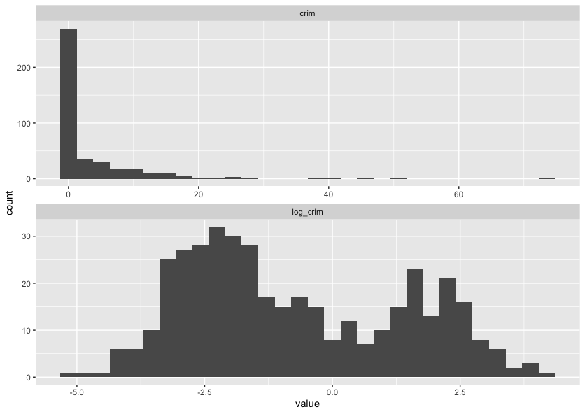
Looking at this graph, it’s likely the log transform of crim will be more useful than the raw values, so rather than manually transforming the data using dplyr::mutate we can add a recipe step to do it for us.
housing_rec <- recipe(medv ~ ., data = housing_train) |>
  step_log(crim) |>
  step_nzv(all_predictors()) |>
  step_normalize(all_numeric_predictors())

housing_rec
── Recipe ───────────────────────────────────────────────────────────────────────────────────────

── Inputs
Number of variables by role
outcome:    1
predictor: 13

── Operations
• Log transformation on: crim
• Sparse, unbalanced variable filter on: all_predictors()
• Centering and scaling for: all_numeric_predictors()
Most of the steps above are for dealing with numeric data, but we commonly have to deal with categorical data too. The most common way of dealing with categorical variables is through dummy variables. This means that if we have a categorical variable with $k$ categories, we create $k - 1$ new variables, one for each category. If an observation is in category $i$, then the $(i-1)$th dummy variable is set to 1 and all other dummy variables are set to 0. If the observation is in the first category though, we set all of the observations to 0, this is called the baseline. This means that we can use these dummy variables as predictors in our model.
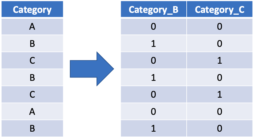
To do this we can use the step_dummy function selecting all_factor_predictors(). This will create dummy variables for all of the categorical predictor variables in our data set.
housing_rec <- recipe(medv ~ ., data = housing_train) |>
  step_log(crim) |>
  step_nzv(all_predictors()) |>
  step_normalize(all_numeric_predictors()) |>
  step_dummy(all_factor_predictors())

housing_rec
── Recipe ───────────────────────────────────────────────────────────────────────────────────────

── Inputs
Number of variables by role
outcome:    1
predictor: 13

── Operations
• Log transformation on: crim
• Sparse, unbalanced variable filter on: all_predictors()
• Centering and scaling for: all_numeric_predictors()
• Dummy variables from: all_factor_predictors()
At this point we should investigate every variable individually and decide what processing this variable will need, both from a machine learning point of view but also using your domain knowledge of where the data came from. There are step specifications for most, if not all, dplyr functions, there are extra packages that contain specifications for lots of different preprocessing steps and it is also possible to write your own.
Perform Your Own Preprocessing
Spend a few minutes now adding a new step to this recipe to perform some data transformation task. This could be as simple as applying a log transform to another variable or you could also look at problems such as missing data (you could look at removing or imputing missing data).
All we have done so far is tell the preprocessor what we would like to do, we haven’t actually fit it yet. We can do this by calling the prep function at the end, which will create a trained data preprocessor that (given the code below) will log the crim variable, not remove any columns (as all of the data has non-zero variance), will subtract the mean value of the training data set from each numeric predictor and will scale each numeric predictor by the standard deviation of the training set.
housing_rec <- recipe(medv ~ ., data = housing_train) |>
  step_log(crim) |>
  step_nzv(all_predictors()) |>
  step_normalize(all_numeric_predictors()) |>
  step_dummy(all_factor_predictors()) |>
  prep()

housing_rec
── Recipe ───────────────────────────────────────────────────────────────────────────────────────

── Inputs
Number of variables by role
outcome:    1
predictor: 13

── Training information
Training data contained 404 data points and no incomplete rows.

── Operations
• Log transformation on: crim | Trained
• Sparse, unbalanced variable filter removed: <none> | Trained
• Centering and scaling for: crim, zn, indus, nox, rm, age, dis, rad, tax, ... | Trained
• Dummy variables from: chas | Trained
To extract the transformed training data from the preprocessor we can use the juice function. This can be useful if you want to retrospectively see if there are any anomolies etc. included in the training data.
juice(housing_rec)
# A tibble: 404 × 14
      crim      zn  indus    nox     rm    age    dis    rad     tax ptratio     b  lstat  medv chas_X1
     <dbl>   <dbl>  <dbl>  <dbl>  <dbl>  <dbl>  <dbl>  <dbl>   <dbl>   <dbl> <dbl>  <dbl> <dbl>   <dbl>
 1 -0.960   0.0643 -0.732 -1.28  -0.609 -1.70   1.34  -0.632 -0.364    0.197 0.445 -0.625  22         0
 2  1.31   -0.487   1.04   1.24  -1.13   1.11  -1.07   1.69   1.55     0.791 0.452  1.66   12.3       0
 3  0.675  -0.487   1.25   0.418  2.37   0.978 -0.819 -0.517 -0.0185  -1.72  0.159 -1.24   50         0
 4 -0.789  -0.487   0.262 -1.03  -0.615 -1.16   0.373 -0.517 -0.0483   0.105 0.443 -0.486  20.3       0
 5  2.03   -0.487   1.04   1.18  -1.23   1.11  -1.09   1.69   1.55     0.791 0.452  2.50    5         0
 6 -1.26   -0.487  -0.861 -0.360 -0.584 -0.335  0.913 -0.517 -1.09     0.791 0.430 -0.283  18.5       0
 7  1.35   -0.487   1.04   1.18   0.253  1.07  -0.975  1.69   1.55     0.791 0.400  0.629  13.1       0
 8  0.0779  0.395  -1.04   0.781  1.32   0.813 -0.876 -0.517 -0.848   -2.50  0.356 -0.625  36.5       0
 9 -1.09    3.04   -1.13  -1.37  -0.741 -1.36   1.40  -0.632 -0.412   -1.08  0.452 -0.328  19.4       0
10 -0.738   0.0643 -0.467 -0.282 -0.593 -1.07   0.834 -0.517 -0.567   -1.49  0.384  0.433  21.7       0
# ℹ 394 more rows
# ℹ Use `print(n = ...)` to see more rows
To transform new data using the data preprocessor we can use the bake function.
bake(housing_rec, housing_test)
# A tibble: 102 × 14
     crim      zn  indus    nox     rm    age     dis    rad    tax ptratio       b  lstat  medv chas_X1
    <dbl>   <dbl>  <dbl>  <dbl>  <dbl>  <dbl>   <dbl>  <dbl>  <dbl>   <dbl>   <dbl>  <dbl> <dbl>   <dbl>
 1 -0.334  0.0643 -0.467 -0.282  0.117  0.910  1.27   -0.517 -0.567 -1.49    0.406   1.09   15         0
 2  0.378 -0.487  -0.428 -0.161 -0.526 -1.42   0.371  -0.632 -0.591  1.16    0.345  -0.837  23.1       0
 3  0.348 -0.487  -0.428 -0.161 -0.703  1.11   0.175  -0.632 -0.591  1.16    0.427   1.01   14.5       0
 4  0.504 -0.487  -0.428 -0.161 -0.504  0.469  0.124  -0.632 -0.591  1.16   -1.30    2.10   13.2       0
 5  0.418 -0.487  -0.428 -0.161 -0.866  0.935  0.0259 -0.632 -0.591  1.16    0.0465  0.800  13.1       0
 6 -0.720 -0.487  -0.748 -0.498 -0.663 -0.270 -0.173  -0.517 -0.758  0.334   0.246  -0.165  20         0
 7 -1.30   2.82   -1.19  -1.11   0.434 -1.69   0.810  -0.748 -0.919 -0.0772  0.439  -1.15   30.8       0
 8 -0.596 -0.487  -0.608 -0.939  0.688 -2.37   0.965  -0.748 -1.03  -0.260   0.330  -1.08   26.6       0
 9 -0.614 -0.487  -0.608 -0.939 -0.331 -1.04   0.965  -0.748 -1.03  -0.260   0.372  -0.424  21.2       0
10 -0.278 -0.487  -0.608 -0.939 -1.31   0.946  1.04   -0.748 -1.03  -0.260   0.452   2.53   14.4       0
# ℹ 92 more rows
# ℹ Use `print(n = ...)` to see more rows
When training a model with tidymodels we don’t actually have to transform (or bake) the data ourselves, we can add this preproceesor to the model worflow and it will automatically be applied when we predict using the model workflow.
Key Points
You can use
rsampleto split your data into training and testing sets.You can use
recipesto create a recipe to preprocess your data.
Building a Simple Workflow
Overview
Teaching: 0 min
Exercises: 0 minQuestions
How do we make a workflow using
tidymodels?Objectives
Create a linear regression workflow using
tidymodels.
Creating a Workflow
As discussed in the introduction, a workflow is a series of steps that are executed in order to accomplish a task, in our case this is to train or make predictions using a model. To initialise a workflow in tidymodels is very simple:
housing_wf <- workflow()

housing_wf
══ Workflow ══════════════════════════════════════════════════════════════════════════════════════════════
Preprocessor: None
Model: None
Here you can see that our workflow object has two slots: a preprocessor and a model. We made a preprocessor object in the last session (our recipe) so we can easily add this to our workflow, we can see our workflow now in the workflow summary and the different preproessing steps involved.
housing_wf <- workflow() |>
  add_recipe(housing_rec)

housing_wf
══ Workflow ══════════════════════════════════════════════════════════════════════════════════════════════
Preprocessor: Recipe
Model: None

── Preprocessor ──────────────────────────────────────────────────────────────────────────────────────────
4 Recipe Steps

• step_log()
• step_nzv()
• step_normalize()
• step_dummy()
Creating a Model
The next thing we need to do is to create a model object to add to the workflow. This is the power of tidymodels as we can create a model object without having to worry about the underlying code. We can create a model object using the linear_reg() function from the parsnip package. This function creates a model object that is a linear regression model.
housing_lin_reg <- linear_reg(
  mode = "regression",
  engine = "lm"
)

housing_lin_reg
Linear Regression Model Specification (regression)

Computational engine: lm
Here you can see we have created a linear regression model object. The mode argument specifies that we want to create a regression model and the engine argument specifies that we want to use the lm function from the stats package to fit the model. For each type of model there are many different implementations of that model (generally different packages implement them slightly differently) and the engine argument allows us to specify which implementation we want to use which can make quite a big difference in some circumstances.
We can also add this to our model and that’s it! We have a workflow that we can use to train a model.
housing_wf <- workflow() |>
  add_recipe(housing_rec) |>
  add_model(housing_lin_reg)

housing_wf
══ Workflow ══════════════════════════════════════════════════════════════════════════════════════════════
Preprocessor: Recipe
Model: linear_reg()

── Preprocessor ──────────────────────────────────────────────────────────────────────────────────────────
4 Recipe Steps

• step_log()
• step_nzv()
• step_normalize()
• step_dummy()

── Model ─────────────────────────────────────────────────────────────────────────────────────────────────
Linear Regression Model Specification (regression)

Computational engine: lm
Fitting a Workflow
Now that we have a workflow we can use it to fit a model. To do this we use the fit() function. This function takes two arguments: the workflow and the data. The data is the data that we want to use to train the model. In this case we want to use the training data that we created in the last session. You can see the coefficients of the model in the output below.
housing_fit <- housing_wf |>
  fit(housing_train)

housing_fit
══ Workflow [trained] ══════════════════════════════════════════════════════════════════════
Preprocessor: Recipe
Model: linear_reg()

── Preprocessor ────────────────────────────────────────────────────────────────────────────
4 Recipe Steps

• step_log()
• step_nzv()
• step_normalize()
• step_dummy()

── Model ───────────────────────────────────────────────────────────────────────────────────

Call:
stats::lm(formula = ..y ~ ., data = data)

Coefficients:
(Intercept)         crim           zn        indus          nox           rm          age
    22.4329       0.8177       0.5474       0.1569      -2.2445       3.1357       0.1204
        dis          rad          tax      ptratio            b        lstat      chas_X1
    -2.4630       1.4247      -1.6586      -2.0529       1.1670      -3.9530       3.2286
Predicting with a Workflow
Now that we have a fitted model we can use it to make predictions. To do this we use the predict() function. This function takes two arguments: the fitted model and the data. The data is the data that we want to use to make predictions. In this case we want to use the test data that we created in a previous session. You can see the predictions of the model in the output below.
housing_res <- housing_fit |>
  predict(housing_train)

housing_res
# A tibble: 404 × 1
   .pred
   <dbl>
 1 21.3
 2 12.0
 3 39.5
 4 22.5
 5  9.16
 6 18.8
 7 20.3
 8 35.9
 9 24.0
10 20.4
# ℹ 394 more rows
# ℹ Use `print(n = ...)` to see more rows
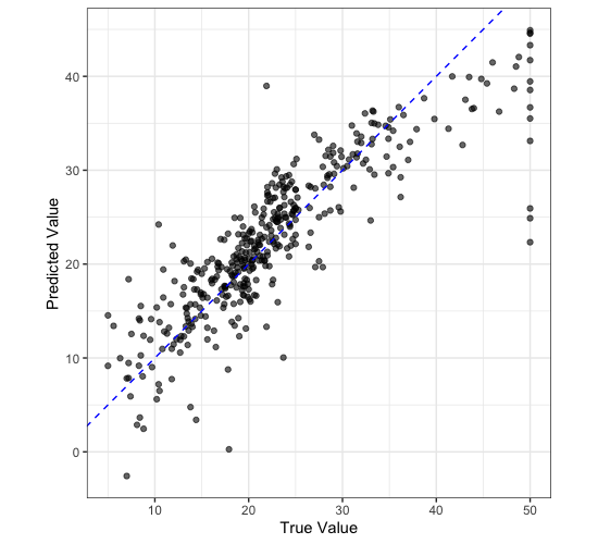
We can plot our predictions against the true values to see how well our model is doing.
housing_train |>
  select(medv) |>
  bind_cols(housing_res) |>
  ggplot() +
  aes(
    x = medv,
    y = .pred
  ) +
  geom_point(
    alpha = 0.6
  ) +
  geom_abline(
    slope = 1,
    colour = "blue",
    lty = 2
  ) +
  labs(
    x = "True Value",
    y = "Predicted Value"
  ) +
  coord_equal() +
  theme_bw()
Key Points
A workflow is a series of steps that are executed in order to accomplish a task.
Hyperparameter Tuning
Overview
Teaching: 0 min
Exercises: 0 minQuestions
How do we tune the hyperparameters of a model?
Objectives
Create a random forest model using
tidymodels.
Hyperparameter Tuning
Linear regression is considered to be a simpler model both due to its constraints and that it has no hyperparameters to tune. If you remember from a previous session, models have parameters and hyperparameters. Parameters are learnt by the model from the data but hyperparameters have to be set by us. Luckily, tidymodels has a lot of tools that we can use for finding the best hyperparameters and justifying the choices we make.
Hyperparameter tuning is performed in tidymodels using a package called dials. We are going to demonstrate how to use dials by training a random forest model, we aren’t going to go into the details of how random forests work but you can see we will be able to train one anyway! When it comes to applying this in the real world, you should always research the model you are using and the basics on how it works to see if it appropriate for your use case.
Identify the Hyperparameters
Use
?rand_forestto look at the help documentation for creating a random forest model. What are the hyperparameters for the model?
Firstly, lets create a new workflow object and add our recipe to it. Note how this is exactly the same as before and we are reusing the same preprocessor
housing_wf_rfrst <- workflow() |>
  add_recipe(housing_rec)
══ Workflow ════════════════════════════════════════════════════════════════════════════════
Preprocessor: Recipe
Model: None

── Preprocessor ────────────────────────────────────────────────────────────────────────────
4 Recipe Steps

• step_log()
• step_nzv()
• step_normalize()
• step_dummy()
Now we can create our model. We are going to use the rand_forest() function from the parsnip package to create a random forest model object. Rather than setting the values of the hyperparameters, we are going to set them equal to the tune() function. This lets tidymodels know that we want to tune these hyperparameters and that this isn’t the final version of the model. You can see that this time we haven’t selected an engine to use but it has defaulted to the ranger package.
housing_rfrst <- rand_forest(
  mode = "regression",
  mtry = tune(),
  trees = tune(),
  min_n = tune()
)

housing_rfrst
Random Forest Model Specification (regression)

Main Arguments:
  mtry = tune()
  trees = tune()
  min_n = tune()

Computational engine: ranger
We can now add this model to our workflow like before.
housing_wf_rfrst <- workflow() |>
  add_recipe(housing_rec) |>
  add_model(housing_rfrst)

housing_wf_rfrst
══ Workflow ════════════════════════════════════════════════════════════════════════════════
Preprocessor: Recipe
Model: rand_forest()

── Preprocessor ────────────────────────────────────────────────────────────────────────────
4 Recipe Steps

• step_log()
• step_nzv()
• step_normalize()
• step_dummy()

── Model ───────────────────────────────────────────────────────────────────────────────────
Random Forest Model Specification (regression)

Main Arguments:
  mtry = tune()
  trees = tune()
  min_n = tune()

Computational engine: ranger
Next we are going to perform cross validation to select the best combination of hyperparameters to use to train the model and to do this we need to decide the combinations to test. Thankfully, tidymodels can do this for us. We can use the extract_parameter_set_dials() to extract the parameters that need tuning from the model as well as what type of parameters they are.
tuning_params <- housing_rfrst |>
  extract_parameter_set_dials()

 tuning_params
Collection of 3 parameters for tuning

 identifier  type    object
       mtry  mtry nparam[?]
      trees trees nparam[+]
      min_n min_n nparam[+]

Model parameters needing finalization:
   # Randomly Selected Predictors ('mtry')

See `?dials::finalize` or `?dials::update.parameters` for more information.
You can see in the output that some hyperparameters need finalization. The tidymodels package is good at guessing different types of parameters but sometimes it needs some extra context. For example, the mtry parameter is the number of randomly selected predictors to use at each split which is dependent in the data set we are using (smaller datasets won’t need as many) and so to get a set of reasonable values we can show the model some example data and it can use this to estimate a good parameter range. We do this using the finalize() function, passing through our training data set.
tuning_params <- housing_rfrst |>
  extract_parameter_set_dials() |>
  finalize(housing_train)

tuning_params
Collection of 3 parameters for tuning

 identifier  type    object
       mtry  mtry nparam[+]
      trees trees nparam[+]
      min_n min_n nparam[+]
Now we can start generating sets of values to test, the simplest method for doing this is using a tuning grid. To create one, a predefined number of values are selected for each hyperparameter and every combination of these values is tested. We do this using the grid_regular() function, passing through the tuning parameters we extracted from the model and the number of values we want to test for each hyperparameter as ‘levels’. There are other, arguably more sophisticated, methods for generating tuning grids, you may wish to try using grid_max_entropy() or grid_latin_hypercube() instead (hint: if you wish to use these you will need to replace the levels argument with size). We are going to use 100 values for each hyperparameter.
tuning_grid <- grid_regular(
  tuning_params,
  levels = 100
)

tuning_grid
# A tibble: 54,600 × 3
    mtry trees min_n
   <int> <int> <int>
 1     1     1     2
 2     2     1     2
 3     3     1     2
 4     4     1     2
 5     5     1     2
 6     6     1     2
 7     7     1     2
 8     8     1     2
 9     9     1     2
10    10     1     2
# ℹ 54,590 more rows
# ℹ Use `print(n = ...)` to see more rows
Now that we have the combinations of hyperparameters that we would like to test we can use the tune_grid() function to train a model with each of these hyperparameter combinations. Rather than passing tune_grid() housing_train we have passed it housing_folds which has the specification for our cross validation sets.
housing_rfrst_tuning <- housing_wf_rfrst |>
  tune_grid(
    housing_folds,
    tuning_params
  )

housing_rfrst_tuning
# Tuning results
# 5-fold cross-validation repeated 3 times
# A tibble: 15 × 5
   splits           id      id2   .metrics          .notes
   <list>           <chr>   <chr> <list>            <list>
 1 <split [323/81]> Repeat1 Fold1 <tibble [20 × 7]> <tibble [0 × 3]>
 2 <split [323/81]> Repeat1 Fold2 <tibble [20 × 7]> <tibble [0 × 3]>
 3 <split [323/81]> Repeat1 Fold3 <tibble [20 × 7]> <tibble [0 × 3]>
 4 <split [323/81]> Repeat1 Fold4 <tibble [20 × 7]> <tibble [0 × 3]>
 5 <split [324/80]> Repeat1 Fold5 <tibble [20 × 7]> <tibble [0 × 3]>
 6 <split [323/81]> Repeat2 Fold1 <tibble [20 × 7]> <tibble [0 × 3]>
 7 <split [323/81]> Repeat2 Fold2 <tibble [20 × 7]> <tibble [0 × 3]>
 8 <split [323/81]> Repeat2 Fold3 <tibble [20 × 7]> <tibble [0 × 3]>
 9 <split [323/81]> Repeat2 Fold4 <tibble [20 × 7]> <tibble [0 × 3]>
10 <split [324/80]> Repeat2 Fold5 <tibble [20 × 7]> <tibble [0 × 3]>
11 <split [323/81]> Repeat3 Fold1 <tibble [20 × 7]> <tibble [0 × 3]>
12 <split [323/81]> Repeat3 Fold2 <tibble [20 × 7]> <tibble [0 × 3]>
13 <split [323/81]> Repeat3 Fold3 <tibble [20 × 7]> <tibble [0 × 3]>
14 <split [323/81]> Repeat3 Fold4 <tibble [20 × 7]> <tibble [0 × 3]>
15 <split [324/80]> Repeat3 Fold5 <tibble [20 × 7]> <tibble [0 × 3]>
This is hard for us to interpret and so we can use the collect_metrics() function to extract the metrics we are interested in.
housing_rfrst_tuning |>
  collect_metrics()
# A tibble: 20 × 9
    mtry trees min_n .metric .estimator  mean     n std_err .config
   <int> <int> <int> <chr>   <chr>      <dbl> <int>   <dbl> <chr>
 1     8  1089    26 rmse    standard   3.35     15  0.186  Preprocessor1_Model01
 2     8  1089    26 rsq     standard   0.869    15  0.0131 Preprocessor1_Model01
 3    11  1384    14 rmse    standard   3.25     15  0.180  Preprocessor1_Model02
 4    11  1384    14 rsq     standard   0.875    15  0.0122 Preprocessor1_Model02
 5     4   309     4 rmse    standard   3.13     15  0.188  Preprocessor1_Model03
 6     4   309     4 rsq     standard   0.889    15  0.0124 Preprocessor1_Model03
 7     6   466    38 rmse    standard   3.56     15  0.195  Preprocessor1_Model04
 8     6   466    38 rsq     standard   0.857    15  0.0144 Preprocessor1_Model04
 9     8  1638    18 rmse    standard   3.26     15  0.186  Preprocessor1_Model05
10     8  1638    18 rsq     standard   0.876    15  0.0127 Preprocessor1_Model05
11     5  1449    33 rmse    standard   3.51     15  0.194  Preprocessor1_Model06
12     5  1449    33 rsq     standard   0.863    15  0.0144 Preprocessor1_Model06
13     3   692    24 rmse    standard   3.61     15  0.197  Preprocessor1_Model07
14     3   692    24 rsq     standard   0.862    15  0.0151 Preprocessor1_Model07
15    12    74    11 rmse    standard   3.24     15  0.178  Preprocessor1_Model08
16    12    74    11 rsq     standard   0.876    15  0.0118 Preprocessor1_Model08
17    10  1824     8 rmse    standard   3.19     15  0.180  Preprocessor1_Model09
18    10  1824     8 rsq     standard   0.880    15  0.0120 Preprocessor1_Model09
19     2   981    30 rmse    standard   4.06     15  0.201  Preprocessor1_Model10
20     2   981    30 rsq     standard   0.833    15  0.0178 Preprocessor1_Model10
We can also quickly create a plot to visualise the results.
autoplot(housing_rfrst_tuning)
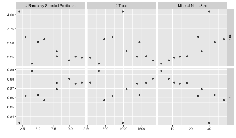
To select the “best” model we can use the select_best() function. We pass these all of the tuning results and the metric we are interested in optimising. In this case we are interested in the model with the highest R-squared.
best_params <- housing_rfrst_tuning |>
  select_best("rsq")

best_params
# A tibble: 1 × 4
   mtry trees min_n .config
  <int> <int> <int> <chr>
1     4   309     4 Preprocessor1_Model03
Now we need set the parameters in our workflow model to be the best parameters we have idenified above. If we take a look at our workflow object, it looks like this
housing_wf_rfrst
══ Workflow ════════════════════════════════════════════════════════════════════════════════
Preprocessor: Recipe
Model: rand_forest()

── Preprocessor ────────────────────────────────────────────────────────────────────────────
4 Recipe Steps

• step_log()
• step_nzv()
• step_normalize()
• step_dummy()

── Model ───────────────────────────────────────────────────────────────────────────────────
Random Forest Model Specification (regression)

Main Arguments:
  mtry = tune()
  trees = tune()
  min_n = tune()

Computational engine: ranger
We can then set the hyperparameters using the finalize_workflow() function. We pass this the workflow object and the best parameters we have identified.
housing_wf_rfrst |>
  finalize_workflow(best_params)
══ Workflow ════════════════════════════════════════════════════════════════════════════════
Preprocessor: Recipe
Model: rand_forest()

── Preprocessor ────────────────────────────────────────────────────────────────────────────
4 Recipe Steps

• step_log()
• step_nzv()
• step_normalize()
• step_dummy()

── Model ───────────────────────────────────────────────────────────────────────────────────
Random Forest Model Specification (regression)

Main Arguments:
  mtry = 4
  trees = 309
  min_n = 4

Computational engine: ranger
As well as finalizing the workflow, we can fit the model to the training data using the fit() function like before and now we have a fully tuned and trained model.
housing_rfrst_fit <- housing_wf_rfrst |>
  finalize_workflow(best_params) |>
  fit(housing_train)


housing_rfrst_fit
══ Workflow [trained] ══════════════════════════════════════════════════════════════════════
Preprocessor: Recipe
Model: rand_forest()

── Preprocessor ────────────────────────────────────────────────────────────────────────────
4 Recipe Steps

• step_log()
• step_nzv()
• step_normalize()
• step_dummy()

── Model ───────────────────────────────────────────────────────────────────────────────────
Ranger result

Call:
 ranger::ranger(x = maybe_data_frame(x), y = y, mtry = min_cols(~4L,      x), num.trees = ~309L, min.node.size = min_rows(~4L, x),      num.threads = 1, verbose = FALSE, seed = sample.int(10^5,          1))

Type:                             Regression
Number of trees:                  309
Sample size:                      404
Number of independent variables:  13
Mtry:                             4
Target node size:                 4
Variable importance mode:         none
Splitrule:                        variance
OOB prediction error (MSE):       9.67719
R squared (OOB):                  0.8873346
Just like before, we can then use the predict() function to generate predictions and then plot the results, as we have seen in the previous section.
housing_rfrst_res <- housing_rfrst_fit |>
  predict(housing_train)

housing_train |>
  select(medv) |>
  bind_cols(housing_res) |>
  ggplot() +
  aes(
    x = medv,
    y = .pred
  ) +
  geom_point(
    alpha = 0.6
  ) +
  geom_abline(
    slope = 1,
    colour = "blue",
    lty = 2
  ) +
  labs(
    x = "True Value",
    y = "Predicted Value"
  ) +
  coord_equal() +
  theme_bw()

This is not the most robust of tests, but to look at how much better our tuned random forest model is compared to the linear regression model we can compare these truth vs. prediction plots.
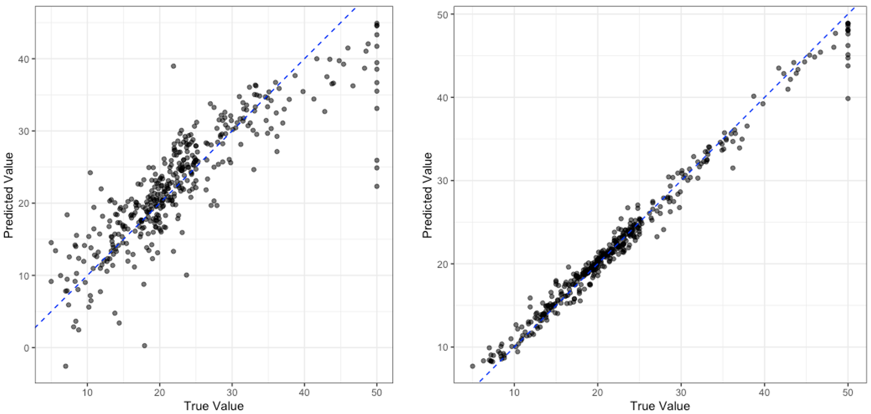
Comparing Models
Which model do you think is performing better? Do you think you can be confident of your answer only using the plot above? Who or why not?
Key Points
Hyperparameters are the settings of a model that we have to set ourselves.
After Training a Model
Overview
Teaching: 0 min
Exercises: 0 minQuestions
How do we test a model?
How do we save and load a model?
Objectives
Test a model on the testing data.
Save and load a model.
Testing a Model
Up until this point we have not touched our testing data, this is good as we should not touch it until after we have performed model selection and training. Once you have a model that you are happy with then you can see how it performs on the testing data to get a idea as to how it will perform in the real world. For this example, we are going to pretend that we have decided we want to use our linear regression model.
So far we have been using the fit() function to fit our model. However, tidymodels has another function called last_fit() which will fit the model to the training data and then test it on the testing data. We can use this function just like we used fit(), but instead of passing in the training data (housing_train) we pass in the training and testing data in the form of the split object we made earlier (housing_split).
housing_lin_reg_last_fit <- housing_wf |>
  last_fit(housing_split)

housing_lin_reg_last_fit
# Resampling results
# Manual resampling
# A tibble: 1 × 6
  splits            id               .metrics         .notes   .predictions       .workflow
  <list>            <chr>            <list>           <list>   <list>             <list>
1 <split [404/102]> train/test split <tibble [2 × 4]> <tibble> <tibble [102 × 4]> <workflow>
This is an object that contains our trained workflow, we can access the workflow by
housing_lin_reg_last_fit |>
  extract_workflow()
══ Workflow [trained] ══════════════════════════════════════════════════════════════════════
Preprocessor: Recipe
Model: linear_reg()

── Preprocessor ────────────────────────────────────────────────────────────────────────────
4 Recipe Steps

• step_log()
• step_nzv()
• step_normalize()
• step_dummy()

── Model ───────────────────────────────────────────────────────────────────────────────────

Call:
stats::lm(formula = ..y ~ ., data = data)

Coefficients:
(Intercept)         crim           zn        indus          nox           rm          age
   22.51650      0.83052      0.96745      0.35432     -2.15434      2.73170     -0.04878
        dis          rad          tax      ptratio            b        lstat      chas_X1
   -2.72384      1.74809     -2.04659     -2.02828      0.99723     -4.26584      2.57621
But the last_fit() function, as well as fitting the model, will evaluate your model on the testing data and provide you with metrics on how well it performed. We can access these metrics by using the collect_metrics() function.
housing_lin_reg_last_fit |>
  collect_metrics()
# A tibble: 2 × 4
  .metric .estimator .estimate .config
  <chr>   <chr>          <dbl> <chr>
1 rmse    standard       3.83  Preprocessor1_Model1
2 rsq     standard       0.791 Preprocessor1_Model1
Is this model any good?
Looking at these metrics, do you think that the model we have trained is any good? Why or why not?
We can also check whether there are any “structural errors” in our model by comparing plots of true and predicted values.
housing_lin_reg_test_res <- housing_lin_reg_last_fit |>
  extract_workflow() |>
  predict(housing_test)

housing_lin_reg_test_res
# A tibble: 102 × 1
   .pred
   <dbl>
 1 20.4
 2 21.7
 3 18.9
 4 16.2
 5 13.9
 6 11.4
 7  8.39
 8 22.8
 9 34.4
10 25.4
# ℹ 92 more rows
# ℹ Use `print(n = ...)` to see more rows
housing_test |>
  select(medv) |>
  bind_cols(housing_lin_reg_test_res) |>
  ggplot() +
  aes(
    x = medv,
    y = .pred
  ) +
  geom_point(
    alpha = 0.6
  ) +
  geom_abline(
    slope = 1,
    colour = "blue",
    lty = 2
  ) +
  labs(
    x = "True Value",
    y = "Predicted Value"
  ) +
  coord_equal() +
  theme_bw()
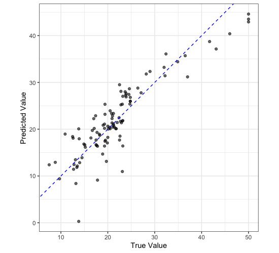
Is this model any good?
Looking at this plot, do you think that the model we have trained is any good? Why or why not?
Saving a Model
Once you have a model that you are happy with, you can save it to disk so that you can use it later. To do this we use the saveRDS() function. The first argument is the object you want to save, the second argument is the path to the file you want to save it to. In this case we are going to save our linear regression model last fit object to a file called model.rds.
saveRDS(
  housing_lin_reg_last_fit,
  "model.rds"
)
We can then read in this model again using the readRDS() function.
model <- readRDS("model.rds")

model |>
  extract_workflow()
══ Workflow [trained] ══════════════════════════════════════════════════════════════════════
Preprocessor: Recipe
Model: linear_reg()

── Preprocessor ────────────────────────────────────────────────────────────────────────────
4 Recipe Steps

• step_log()
• step_nzv()
• step_normalize()
• step_dummy()

── Model ───────────────────────────────────────────────────────────────────────────────────

Call:
stats::lm(formula = ..y ~ ., data = data)

Coefficients:
(Intercept)         crim           zn        indus          nox           rm          age
   22.51650      0.83052      0.96745      0.35432     -2.15434      2.73170     -0.04878
        dis          rad          tax      ptratio            b        lstat      chas_X1
   -2.72384      1.74809     -2.04659     -2.02828      0.99723     -4.26584      2.57621
Key Points
We can use
last_fit()to test a model on the testing data.We can use
saveRDS()andreadRDS()to save and load a model.
Full Walkthrough For Classification
Overview
Teaching: 0 min
Exercises: 0 minQuestions
Can we apply what we have learnt to a new dataset?
Objectives
Apply what we have learnt to a new dataset.
data <- iris |>
  as_tibble()

data_split <- initial_split(data, prop = 0.8, strata = Species)
data_train <- training(data_split)
data_test <- testing(data_split)

data_folds <- vfold_cv(data_train, repeats = 5, strata = Species)

data_rec <- recipe(Species ~ ., data = data_train) |>
  step_normalize(all_numeric()) |>
  prep()

data_knn <- nearest_neighbor(
  mode = "classification",
  neighbors = tune(),
  weight_func = tune(),
  dist_power = tune()
)

data_wf <- workflow() |>
  add_recipe(data_rec) |>
  add_model(data_knn)

tuning_params <- data_knn |>
  extract_parameter_set_dials()

data_tuning_grid <- grid_latin_hypercube(
  tuning_params,
  size = 100
)

data_tune <- tune_grid(
  data_wf,
  data_folds,
  tuning_params
)

data_tune |>
  collect_metrics()

autoplot(data_tune)

best_params <- data_tune |>
  select_best("roc_auc")

data_last_fit <- data_wf |>
  finalize_workflow(best_params) |>
  last_fit(data_split)

data_last_fit |>
  collect_metrics()

iris_test_res <- data_test |>
  select(Species) |>
  bind_cols(
    data_last_fit |>
      extract_workflow() |>
      predict(data_test)
  ) |>
  transmute(
    ref = Species,
    pred = .pred_class
  )

library(caret)

confusionMatrix(data = iris_test_res$pred, reference = iris_test_res$ref)
Confusion Matrix and Statistics

            Reference
Prediction   setosa versicolor virginica
  setosa         10          0         0
  versicolor      0          8         2
  virginica       0          2         8

Overall Statistics

               Accuracy : 0.8667
                 95% CI : (0.6928, 0.9624)
    No Information Rate : 0.3333
    P-Value [Acc > NIR] : 2.296e-09

                  Kappa : 0.8

 Mcnemar's Test P-Value : NA

Statistics by Class:

                     Class: setosa Class: versicolor Class: virginica
Sensitivity                 1.0000            0.8000           0.8000
Specificity                 1.0000            0.9000           0.9000
Pos Pred Value              1.0000            0.8000           0.8000
Neg Pred Value              1.0000            0.9000           0.9000
Prevalence                  0.3333            0.3333           0.3333
Detection Rate              0.3333            0.2667           0.2667
Detection Prevalence        0.3333            0.3333           0.3333
Balanced Accuracy           1.0000            0.8500           0.8500
Key Points
We can apply what we have learnt to a new dataset.